Handling Dates In Excel
Because the standard Gregorian calendar used by the majority of the world doesn’t lend itself to date calculations (differing length months, and leap years to name but two examples), Microsoft have devised a special system for dates within Excel which makes it easy to incorporate calculations based on dates into your spreadsheets and Excel based applications.
Excel stores it’s date in a sequential fashion with the number 1 representing January 1st 1900, and all other numbers are either positive or negative based on that date, in increments of 1 per day. So the number 24637 represents 15th June 1967 as this date is 24637 days after 1st January 1900.
Where times are involved, Excel will quote this as decimal fractions of a day, with the day starting at midnight. So 6am on the 15th June 1967 would be quoted as 24637.25 as it’s ¼ of the day extra to 15th June 1967.
Once we have an appreciation of how Excel handles its dates, it then becomes quite easy to do some calculations based on this:
On a blank worksheet, enter text in Cells A1, A2, and D2 as shown below.
Now enter dates in B1 and B2 as shown below – (You will need to type the year of 1900 in full, see ‘Top Tips’ for more information)
Now we need to calculate the number of days elapsed between the two days, so in cell B4 enter the formula B2-B1, and you will see the result shown below.
Whilst this at first appears to be an odd result it’s actually quite logical, Excel has taken the numeric value for 15/06/1967, and subtracted from it the numeric value for 15/06/1900, and inserted the result into Cell B3, because Excel has dealt with dates as part of the calculation it has formatted the cell to contain a date.
Re-formatting the cells to number format, (by selecting Tools –> Cells –> Format) will change the cell, and display the number of days between the two dates specified as shown below.
Formatting Dates
Under the ‘Format Cells’ dialog there are various options for changing the way that cells containing dates are displayed, by changing these a date such as 15th June 1967 can be displayed in various fashions such as;
- 15 June 1967
- 15/06/67
- 15/06/1967
- 1967/06/15
Careful consideration should be given to the format of date cells as the wrong format can cause confusion especially if a workbook is shared internationally.
Using the ‘Weekday’ function
When designing an application that utilises dates, it is often useful to be able to know what day of the week a particular date falls on. Excel provides this functionality through its ‘Weekday’ function.
Using the example shown above, to show the day of the week in the cells adjacent to the dates we need to add the following formulae:
In cell C1 add: =TEXT(WEEKDAY(B1),”dddd”)
In cell C2 add: =TEXT(WEEKDAY(B2),”dddd”)
And you will see the text ‘Friday’ and ‘Thursday’ in cell C1 & C2. Changing the dates in the cells then changes the day of the week correspondingly. In the formula, the Weekday function returns the number of the day of the week that this date falls on, the Text function turns this is into the actual text of the day of the week, and the “dddd” switch shows that the day is to be displayed in full (To use the shortened version of the day change it to “ddd” and the days will show as ‘Fri’ & ‘Thu’
Simple Date Calculations in Excel
Excel has some nice, and easy to use functions that allow you to calculate the number of days, months, and years between two dates, the easiest way to explain this is with some examples
In these examples we will assume that there is a fixed date in cell A1, and we want to calculate the difference between then and now, of various aspects:
To calculate the number of days between two dates use the formula:
=DATEDIF(A1,TODAY(),”d”)
To calculate the number of months between two dates use the formula:
=DATEDIF(A1,TODAY(),”m”)
To calculate the number of whole years between two dates use the formula:
=DATEDIF(A1,TODAY(),”y”)
To calculate the number of years (with a decimal) between the two dates use the formula
=DATEDIF(A1,TODAY(),”m”)/12
Of course if you have two cells with dates in them you can calculate the differences based on those by replacing TODAY() with the appropriate cell reference.


